These are some notes I took while studying diffusion models. I already implemented this paper on PyTorch.

Introduction

The ideal for generating images would be to define a probabilistic distribution containing all image content, and after that generate the image through a random process based on weighted probability as LLM does. But this is a huge task, and at the moment it is not possible.

Diffusion models propose a process to achieve image generation thoug a similar method: to develop a neural network-based model that is able to gradually remove Gaussian noise from an image. So starting from any image generaeted through a Gaussian noise distribution $\mathcal{N}(0, 1)$, converge to image space after a finite number of $\mathcal{N}(0, 1)$ steps.

Noising Process

To train this type of model, the first step is to develop an algorithm that takes any image and converts it to white noise in a finite number of steps. This will act as a starting point for our model which we will train to do the reverse process.

Initial approach

One method that could be considered is to simply add white noise step by step:

$$x_{t} = x_{t-1} + \beta \cdot \epsilon$$ $$x_{t} = x_{0} + \sqrt{t} \cdot \beta \cdot \epsilon$$

---

Notation:

• $x_0$ refers to the original image
• $x_t$ image adter applying t-steps of noising
• $\beta$ corresponds to the weight of noise
• $\epsilon \sim \mathcal{N}(0, 1)$ is the noise added each step generated throug a normal distribution

---

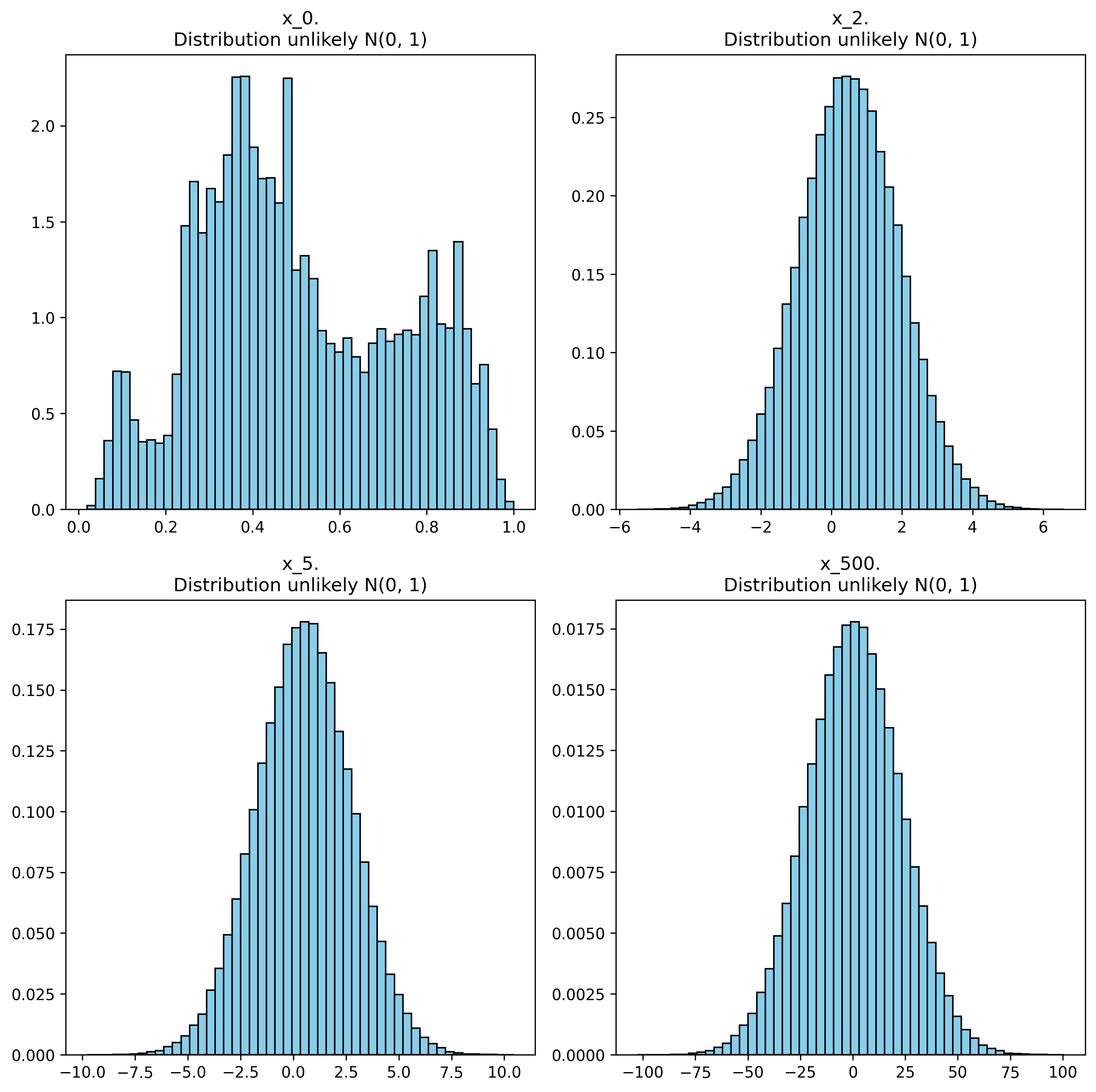
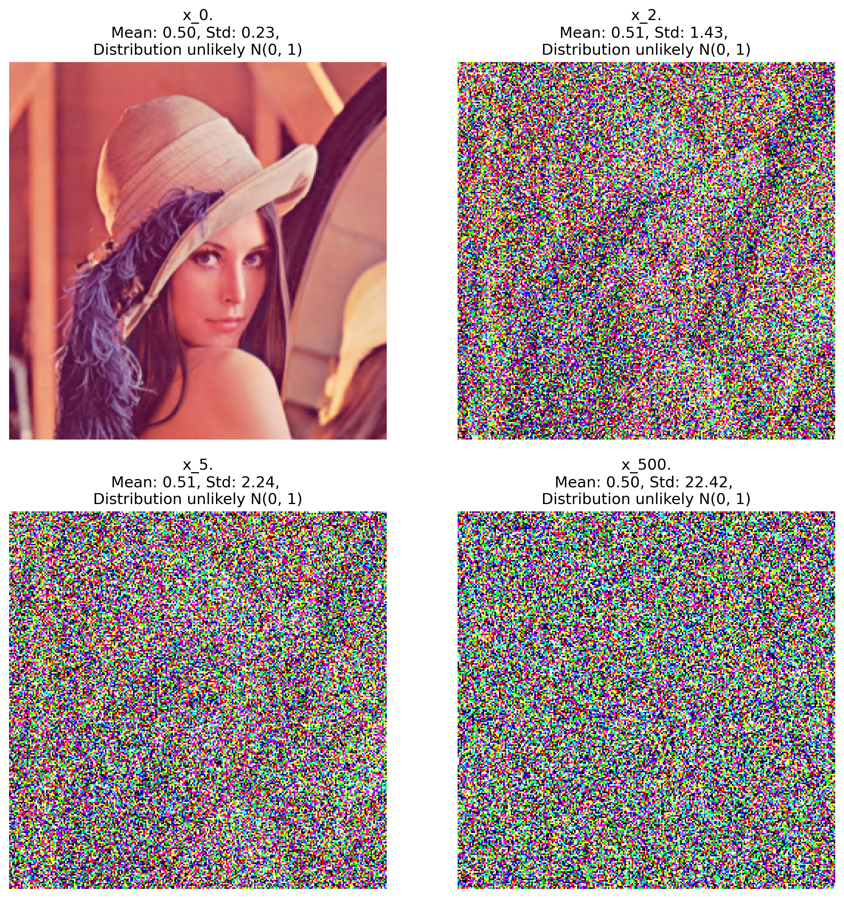
Noising process example on an image over 500 steps. For testing if each distribution was likely a $\mathcal{N}(0, 1)$ distribution, it was applied Kolmogorov-Smirnov test.

The problem with this method is that the distribution diverges at:

$$\lim_{t \to \infty} x_t \sim \lim_{\sigma \to \infty} \mathcal{N}(0, \sigma^2)$$

This phenomenon is called variance exploitation.

Noising process example on an image over 500 steps. For testing if each distribution was likely a $\mathcal{N}(0, 1)$ distribution, it was applied Kolmogorov-Smirnov test.

Diffusion method

An alternative method is proposed in the original paper:

$$x_{t} = \sqrt{\alpha_t} \cdot x_{t-1} + \sqrt{1 - \alpha_t} \cdot \epsilon_t$$ $$x_{t} = \sqrt{\bar{\alpha_t}} \cdot x_{0} + \sqrt{1 - \bar{\alpha_t}} \cdot \epsilon$$

With $\alpha_t = 1 - \beta_t, \space \space \space \bar{\alpha_t} = \prod_{s=1}^{t} \alpha_s$.

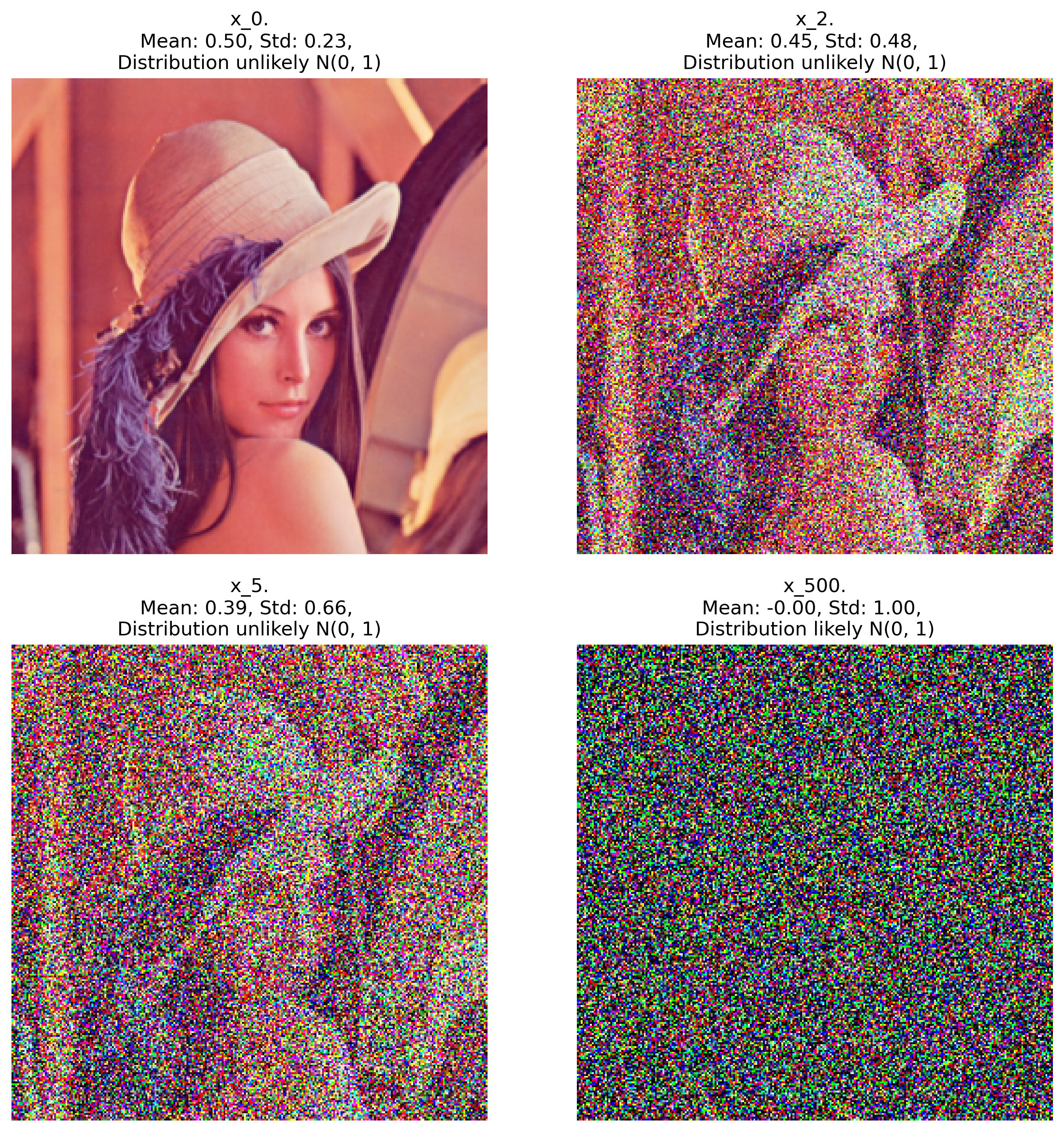
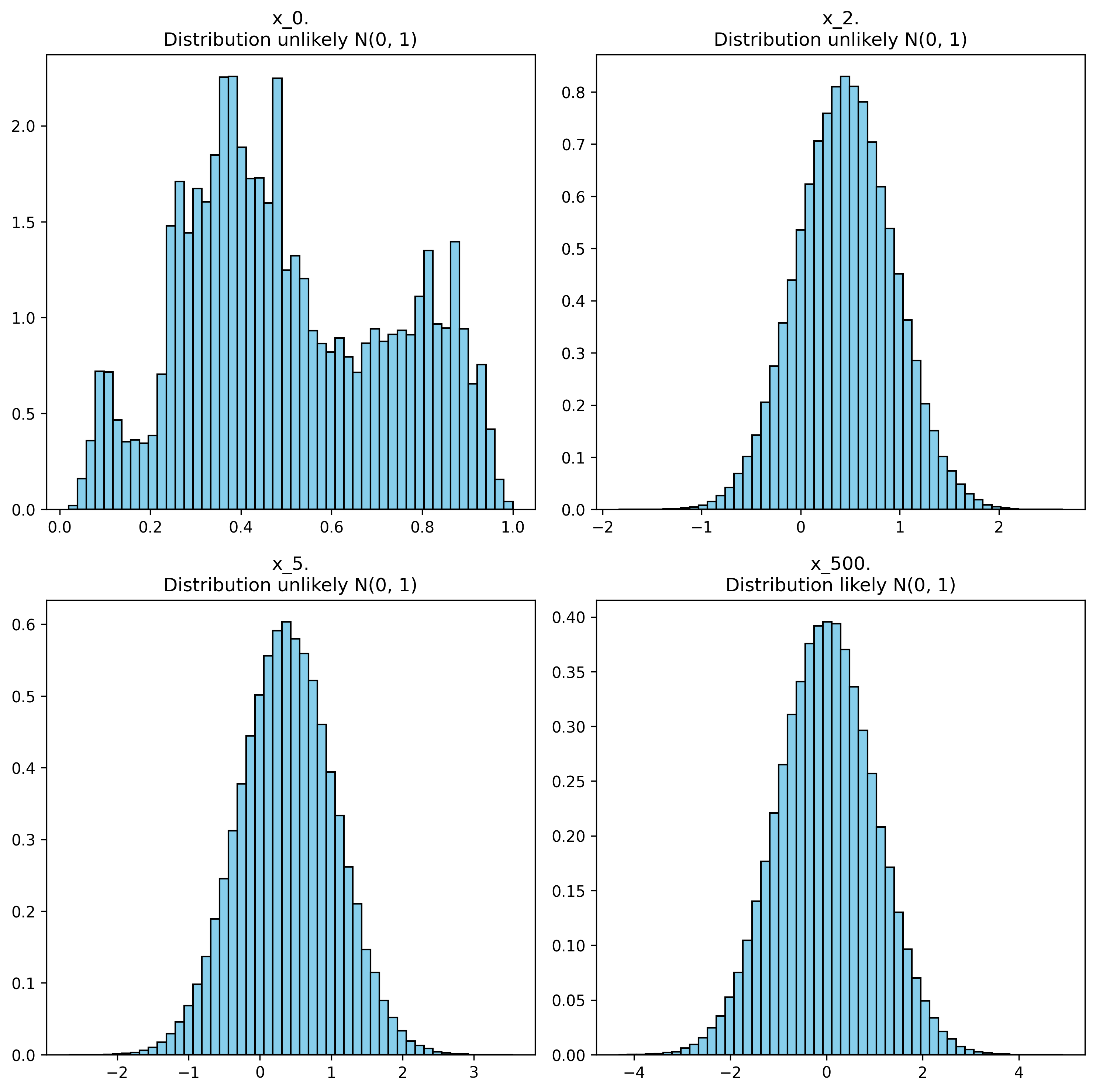
Diffusion process example on an image over 500 steps. For testing if each distribution was likely a $\mathcal{N}(0, 1)$ distribution, it was applied Kolmogorov-Smirnov test.

It could be shown that this distribution already converges to a normal distribution:

$$\lim_{t \to \infty} x_t \sim \mathcal{N}(0, 1)$$

Diffusion process example on an image over 500 steps. For testing if each distribution was likely a $\mathcal{N}(0, 1)$ distribution, it was applied Kolmogorov-Smirnov test.

We have already defined a successful method that converges to a standardized normal distribution.

Markov chain notation

The forward process or diffusion process is defined as a Markov chain:

$$q(x_{1}x_{2}...x_{T}|x_{0}) = q(x_{1:T}|x_{0}) = \prod_{t=1}^{T} q(x_{t}|x_{t-1})$$

Where q is the probability density function of obtaining the value $x_t$ from the value $x_{t-1}$.

$$q(x_t \mid x_{t-1}) = \mathcal{N}(x_t; \sqrt{1 - \beta_t} \cdot x_{t-1}, \beta_t I)$$

---

Notation:

$\mathcal{N}(x, \mu, \sigma)$ refers to the density probability function of normal distribution having the value x. To obtain the probability it must be integrated over the entire image space.

$$Q(x_{1:T}|x_{0}) = \int \prod_{t=1}^{T} q(x_{t}|x_{t-1}) dx_{1:T}$$

---

Denoising Process

The inverse process is defined as the denoising process that converts a denoised image $x_T$ into a functional image. The whole process can be defined as a Markov chain:

$$p_{\theta}(x_{0:T}) = p_{\theta}(x_{T}) \prod_{t=1}^{T}p_{\theta}(x_{t-1}|x_{t})$$

Since by definition it starts from white noise, probability of the initial noise state could be considered as:

$$p_{\theta}(x_{T}) = \mathcal{N}(x_{T}, 0, I)$$

---

Notation:

$\theta$ refers to the parameters of the neural network. If any element contains $\theta$ it means that it was calculated through NN and its parameters.

---

By definition $p_\theta$ and $q$ are inverse processes of themselves. It can be shown that the inverse process of a Gaussian is a Gaussian (reference to demonstration) so:

$$p_{\theta}(x_{t-1}|x_{t}) = \mathcal{N}(x_{t-1}, \mu_{\theta}(x_{t}, t), \sigma_{\theta}(x_{t}, t))$$

Loss Function

Now that we have defined the stochastic process, it is time to define the loss function, as we have a probability density function over images, higer the probability of a generated image it is, better the image it is. Taking this into account the loss function could be defined as:

$$\mathcal{L}= \mathbb{E}[-\log p_\theta (x_0)]$$

With $\mathbb{E}$ referred as the mean value over all the examples and $p_\theta(x_0)$ could be obtained by integrating:

$$p_\theta(x_0) = \int p_\theta(x_{0:T}) dx_{1:T}$$

Since it is not computationally possible to integrate over all the values, an approximation based on Jensen’s inequality is made.

Evidence lower bound (ELBO)

From an equation:

$$\log p(x) = \log \int p(x, z) dz = \log \int q(z \mid x) \frac{p(x, z)}{q(z \mid x)} dz$$

Applying Jensen Inequality (for convex functions):

$$f(\mathbb{E}[X]) \ge \mathbb{E}[f(X)]$$ $$\log p(x) \ge \log \int q(z \mid x) \frac{p(x, z)}{q(z \mid x)} dz$$

Resulting in what is known as the ELBO function:

$$\text{ELBO}(x) = \mathbb{E}_{q(z \mid x)} [\log p(x, z) - \log q(z \mid x)]$$

This applied to the previous defined loss function:

$$\mathcal{L} = \mathbb{E}_q[-\log \frac{p_\theta(x_{0:T})}{q(x_{1:T}\mid x_0))}] \ge \mathbb{E}[-\log p_\theta(x_0)]$$

Using log function properties:

$$\mathcal{L} = \mathbb{E}_q [-\log \frac{p_{\theta}(x_{T}) \prod_{t=1}^{T}p_{\theta}(x_{t-1}|x_{t})}{\prod_{t=1}^{T} q(x_{t}|x_{t-1})} ]$$ $$= \mathbb{E}_q [-\log p_{\theta}(x_{T}) - \sum_{t=1}^{T} \log \frac{p_{\theta}(x_{t-1}|x_{t})}{q(x_{t}|x_{t-1})} ]$$ $$= \mathbb{E}_q [-\log\frac{p_\theta(x_T)}{q(x_T \mid x_0)} - \sum_{t>1}^{T} \log \frac{p_{\theta}(x_{t-1}|x_{t})}{q(x_{t-1}|x_{t},x_0)} - \log p_\theta (x_0 \mid x_1) ]$$ $$= \mathbb{E}_q [D_{\text{KL}}(q(x_T \mid x_0) \mid\mid p_\theta(x_T)) + \sum_{t>1}^{T} D_{\text{KL}}(q(x_{t-1}|x_{t},x_0)\mid\mid p_{\theta}(x_{t-1}|x_{t})) - \log p_\theta (x_0 \mid x_1) ]$$ $$= \mathcal{L}_T + \sum_{t>1}^{T} \mathcal{L}_{t-1} + \mathcal{L}_0$$

Where the new terms that depend on the original image are defined by Bayes theorem as:

$$q(x_{t−1} \mid x_t, x_0) \propto q(x_t \mid x_{t−1}) q(x_{t−1} \mid x_0)$$ $$q(x_{t-1} \mid x_t, x_0) = \mathcal{N}\left(x_{t-1}; \mu_t(x_t, x_0), \tilde{\beta}_t I \right)$$

Where:

$$\mu_t(x_t, x_0) = \frac{\sqrt{\bar{\alpha}_{t-1}} \, \beta_t}{1 - \bar{\alpha}_t} x_0 + \frac{\sqrt{\alpha_t} (1 - \bar{\alpha}_{t-1})}{1 - \bar{\alpha}_t} x_t$$ $$\tilde{\beta}_t = \frac{1 - \bar{\alpha}_{t-1}}{1 - \bar{\alpha}_t} \beta_t$$

Computing Divergence of 2 Gaussians

As every distribution is considered gaussian, computing the divergence would be:

$$D_{\text{KL}}(p \mid\mid q) = \int_{-\infty}^{+\infty} p(x) \log\frac{p(x)}{q(x)} dx$$ $$D_{KL}(p \| q) = \frac{1}{2} \left[\log \frac{|\Sigma_q|}{|\Sigma_p|} - d + \mathrm{tr}(\Sigma_q^{-1} \Sigma_p) + (\mu_p - \mu_q)^T \Sigma_q^{-1} (\mu_p - \mu_q)\right]$$

But the mean and deviation of the distributions are not known, so we have to stimate through numeric methods.

An approach that could be used is Monte Carlo

$$D_{KL}(p \| q) = \mathbb{E}_{x \sim p} \left[ \log \frac{p(x)}{q(x)} \right] \approx \frac{1}{N} \sum_{i=1}^N \log \frac{p(x_i)}{q(x_i)}, \; x_i \sim p$$

But computing it though this methods add a high variance so it is computed thoug Rao-Blackwellized fashion:

$$D_{KL}(p \| q) = \mathbb{E}_{x \sim p} \left[ \log \frac{p(x)}{q(x)} \right] = \mathbb{E}_{x_1} \left[ \mathbb{E}_{x_2 \mid x_1} \left[ \log \frac{p(x_1, x_2)}{q(x_1, x_2)} \right] \right]$$

By numeric methods:

$$D_{KL}(p \| q) \approx \frac{1}{N} \sum_{i=1}^{N} g(x_1^{(i)})$$ $$g(x_1^{(i)}) = \log \frac{p(x_1^{(i)})}{q(x_1^{(i)})} + D_{KL}(p(x_2 \mid x_1^{(i)}) \| q(x_2 \mid x_1^{(i)}))$$

Analyzing loss function

Noised image contribution

$$\mathcal{L}_T = D_{\text{KL}}(q(x_T \mid x_0) \mid\mid p_\theta(x_T))$$

As $x_T$ is generated thoug a normal standard distribution and no apportation of NN weights to the computation of this loss and we consider as hyperparameters $\beta_t$ in terms of model optimizaation we consider $\mathcal{L}_T$ as a constant loss function in terms of $\theta$.

Noising process contribution

$$\mathcal{L}_{t-1} = D_{\text{KL}}(q(x_{t-1}|x_{t},x_0)\mid\mid p_{\theta}(x_{t-1}|x_{t}))$$

As working with normal distributions is easier, it is considered that both distributions are gaussians:

$$q(x_{t-1}|x_{t},x_0) = \mathcal{N}(\mu_\theta, \sigma_\theta)$$ $$p_{\theta}(x_{t-1}|x_{t}) = \mathcal{N}(\tilde{\mu_t}, \tilde{\beta_t})$$

Now divergence results as simple as (considering $\sigma_\theta$ constant for ovidding overfitting):

$$\mathcal{L}_{t-1} = D_{\text{KL}}\left( \mathcal{N}(\mu_\theta, \sigma^2) \,\|\, \mathcal{N}(\tilde{\mu}_t, \sigma^2) \right) = \frac{1}{2\sigma^2} \left\| \tilde{\mu}_t - \mu_\theta \right\|^2$$

Denoised image contribution

If we suppose that we are working with unit8 images, each pixel contains a number between 0 and 255, we are going to work with this values normalized into the interval [-1, 1]. If we consider a pixel discrete pixel value into a continues space we should consider:

$$x \rightarrow [x - \frac{1}{255}, x + \frac{1}{255}]$$

This transformation fully transforms discrete pixel values into continous space. For completion into the real space, we consider in limits intervals: $(+\infty, x + \frac{1}{255}]$ and $[x - \frac{1}{255}, +\infty)$.

So the result of conditioned probability would be the integral over each pixel (and channel) $D$:

$$p_\theta (x_0 \mid x_1) = \prod_{d=1}^{D}\int_{\delta_-(x_0^d)}^{\delta_-(x_0^d)} \mathcal{N} (x; \mu_\theta(x_1, 1), \sigma_{1}^{2} I) dx$$ $$\delta_+(x) = \begin{cases}x + \frac{1}{255} & \text{if } x < 1 \\+\infty & \text{if } x = 1\end{cases}, \quad \delta_-(x) = \begin{cases}x - \frac{1}{255} & \text{if } x > -1 \\-\infty & \text{if } x = -1\end{cases}$$

Observation: For generating less biased models finally only $\mu_\theta$ depends on the model parameter model deviation is not considered.

Simplified loss function

As we previously said, $\mathcal{L}_T$ is not dependant on $\theta$. As the amount of steps is in order of 500, we are not considering anymore $\mathcal{L}_0$.

$$\mathcal{L} \approx \sum_{t=1}^{T} \mathcal{L}_{t-1} = \mathbb{E}_{q,t} \left [ \frac{\beta_{t}^{2}} {2 \sigma_t^2 \alpha_t (1 - \bar{\alpha_t})} \left\| \epsilon - \epsilon _\theta (x_t, t) \right\|^{2} \right ]$$

The loss function is trained to be able to predict the noise that was added to an image at any step.

Training loop

1. Sample $x_0 \sim q(x_0)$

2. Sample $t \sim \text{Uniform}(\{1, \dots, T\})$

3. Sample $\epsilon \sim \mathcal{N}(0, I)$

4. Compute the noised image

   $x_t = \sqrt{\bar{\alpha}_t}x_0 + \sqrt{1 - \bar{\alpha}_t}\epsilon$

5. Take gradient descent step on the difference between the predicted noise and the actual noise

   $\nabla_\theta \big\| \epsilon - \epsilon_\theta(x_t\, t) \big\|^2$

Generation loop

1. Sample $x_T \sim \mathcal{N}(\textbf{0}, \textbf{I})$

2. for t = T, …, 1 do

3.    Sample $z \sim \mathcal{N}(\textbf{0}, \textbf{I}) \text{ if } t > 1 \text{ else } z = \textbf{0}$

4.    Compute the denoised image

   $x_{t-1} = \frac{1}{\sqrt{\alpha_t}} \left( x_t - \frac{1 - \alpha_t}{\sqrt{1 - \bar{\alpha}_t}} \, \varepsilon_\theta(x_t, t) \right) + \sigma_t z$

5. endfor

Resources

• Denoising Diffusion Probabilistic Models (DDPM) – The original paper by Ho et al. that introduced diffusion models for generative modeling.
• How Diffusion Models Work – A visual and intuitive YouTube explanation of how diffusion models function.